# Import pandas and numpy

import pandas as pd
import numpy as np

df = pd.read_csv('2017_Yellow_Taxi_Trip_Data.csv')Google Advanced Data Analytics Certification: Exploratory Data Analysis
Python
EDA
Note
This is taken from the Google Advanced Data Analytics Certification. I am using this as a way to practice my data analysis skills. The code chunks follow a series of prompts. The code to clean and explore the data was generated by me using the instructions provided.
Course 2 End-of-course project:
Inspect and analyze data
Prompt: You have just started as a data professional in a fictional data consulting firm, Automatidata. Their client, the New York City Taxi and Limousine Commission (New York City TLC), has hired the Automatidata team for its reputation in helping their clients develop data-based solutions.
The team is still in the early stages of the project. Previously, you were asked to complete a project proposal by your supervisor, DeShawn Washington. You have received notice that your project proposal has been approved and that New York City TLC has given the Automatidata team access to their data. To get clear insights, New York TLC’s data must be analyzed, key variables identified, and the dataset ensured it is ready for analysis.
In this activity, you will examine data provided and prepare it for analysis. This activity will help ensure the information is,
Ready to answer questions and yield insights
Ready for visualizations
Ready for future hypothesis testing and statistical methods
The purpose of this project is to investigate and understand the data provided.
The goal is to use a dataframe contructed within Python, perform a cursory inspection of the provided dataset, and inform team members of your findings.
This activity has three parts:
Part 1: Understand the situation
- Prepare to understand and organize the provided taxi cab dataset and information.
Part 2: Understand the data
Create a pandas dataframe for data learning, future exploratory data analysis (EDA), and statistical activities.
Compile summary information about the data to inform next steps.
Part 3: Understand the variables
- Use insights from your examination of the summary data to guide deeper investigation into specific variables.
Follow the instructions and answer the following questions to complete the activity. Then, you will complete an Executive Summary using the questions listed on the PACE Strategy Document.
Be sure to complete this activity before moving on. The next course item will provide you with a completed exemplar to compare to your own work.
Task 1. Understand the situation
How can you best prepare to understand and organize the provided taxi cab information?
- Answer:
I can best prepare to understand and organize the provided taxi cab information by first reading the data dictionary and then creating a dataframe in Python.
- Answer:
Task 2a. Build dataframe
Create a pandas dataframe for data learning, and future exploratory data analysis (EDA) and statistical activities.
Code the following,
import pandas as
pd. pandas is used for buidling dataframes.import numpy as
np. numpy is imported with pandasdf = pd.read_csv()
Task 2b. Understand the data - Inspect the data
View and inspect summary information about the dataframe by coding the following:
df.head(10)
df.info()
df.describe()
Consider the following two questions:
Question 1: When reviewing the df.info() output, what do you notice about the different variables? Are there any null values? Are all of the variables numeric? Does anything else stand out?
df.head(10) Unnamed: 0 VendorID ... improvement_surcharge total_amount
0 24870114 2 ... 0.3 16.56
1 35634249 1 ... 0.3 20.80
2 106203690 1 ... 0.3 8.75
3 38942136 2 ... 0.3 27.69
4 30841670 2 ... 0.3 17.80
5 23345809 2 ... 0.3 12.36
6 37660487 2 ... 0.3 59.16
7 69059411 2 ... 0.3 19.58
8 8433159 2 ... 0.3 9.80
9 95294817 1 ... 0.3 16.55
[10 rows x 18 columns]df.info()<class 'pandas.core.frame.DataFrame'>
RangeIndex: 22699 entries, 0 to 22698
Data columns (total 18 columns):
# Column Non-Null Count Dtype
--- ------ -------------- -----
0 Unnamed: 0 22699 non-null int64
1 VendorID 22699 non-null int64
2 tpep_pickup_datetime 22699 non-null object
3 tpep_dropoff_datetime 22699 non-null object
4 passenger_count 22699 non-null int64
5 trip_distance 22699 non-null float64
6 RatecodeID 22699 non-null int64
7 store_and_fwd_flag 22699 non-null object
8 PULocationID 22699 non-null int64
9 DOLocationID 22699 non-null int64
10 payment_type 22699 non-null int64
11 fare_amount 22699 non-null float64
12 extra 22699 non-null float64
13 mta_tax 22699 non-null float64
14 tip_amount 22699 non-null float64
15 tolls_amount 22699 non-null float64
16 improvement_surcharge 22699 non-null float64
17 total_amount 22699 non-null float64
dtypes: float64(8), int64(7), object(3)
memory usage: 3.1+ MB- Answer:
When reviewing the df.info() output, I notice that there are 18 columns and 22,699 rows. I also notice that there are no null values. All of the variables are numeric with the exception of two date-time variables and one categorical variable.
Question 2: When reviewing the df.describe() output, what do you notice about the distributions of each variable? Are there any questionable values?
df.describe() Unnamed: 0 VendorID ... improvement_surcharge total_amount
count 2.269900e+04 22699.000000 ... 22699.000000 22699.000000
mean 5.675849e+07 1.556236 ... 0.299551 16.310502
std 3.274493e+07 0.496838 ... 0.015673 16.097295
min 1.212700e+04 1.000000 ... -0.300000 -120.300000
25% 2.852056e+07 1.000000 ... 0.300000 8.750000
50% 5.673150e+07 2.000000 ... 0.300000 11.800000
75% 8.537452e+07 2.000000 ... 0.300000 17.800000
max 1.134863e+08 2.000000 ... 0.300000 1200.290000
[8 rows x 15 columns]- Answer:
When reviewing the df.describe() output, I notice that the minimum value for the trip_distance variable is 0.00. This is a questionable value because it is not possible to have a trip distance of 0.00. The trip distance has an outlier of 33 miles. The fare amount has negative values. The tip amount has an max of $200, well above the IQR.
Task 2c. Understand the data - Investigate the variables
Sort and interpret the data table for two variables:trip_distance and total_amount.
Answer the following three questions:
Question 1: Sort your first variable (trip_distance) from maximum to minimum value, do the values seem normal?
df.sort_values(by=['trip_distance'], ascending=False)['trip_distance']9280 33.96
13861 33.92
6064 32.72
10291 31.95
29 30.83
...
13359 0.00
21194 0.00
246 0.00
15084 0.00
8353 0.00
Name: trip_distance, Length: 22699, dtype: float64- Answer:
When sorting the trip_distance variable from maximum to minimum value, the values do not seem normal. The maximum value is 33 miles, and there are others well above the 1.5*IQR threshold, which qualifies them as an outlier. The minimum value is 0.00 miles, which is not possible.
Question 2: Sort by your second variable (total_amount), are any values unusual?
df.sort_values(['trip_distance'], ascending = False)[['total_amount','trip_distance']] total_amount trip_distance
9280 150.30 33.96
13861 258.21 33.92
6064 179.06 32.72
10291 131.80 31.95
29 111.38 30.83
... ... ...
13359 111.95 0.00
21194 3.80 0.00
246 3.80 0.00
15084 4.80 0.00
8353 3.30 0.00
[22699 rows x 2 columns]- Answer:
There is one value above $1,000, and there are negative values. The negative values bring into question the validity of the data.
Question 3: Are the resulting rows similar for both sorts? Why or why not?
- Answer:
Not exactly. The $1200 trip was for 2.60 miles. The 33.92 mile trip was $258.21, which might be reasonable.
According to the data dictionary, the payment method was encoded as follows:
1 = Credit card
2 = Cash
3 = No charge
4 = Dispute
5 = Unknown
6 = Voided trip
- How many of each payment type are represented in the data?
df['payment_type'].value_counts()payment_type
1 15265
2 7267
3 121
4 46
Name: count, dtype: int64- What is the average tip for trips paid for with credit card?
avg_cc_tip = df[df['payment_type']==1]['tip_amount'].mean()
print('Avg. cc tip:', avg_cc_tip)
Avg. cc tip: 2.7298001965280054- What is the average tip for trips paid for with cash?
avg_cash_tip = df[df['payment_type']==2]['tip_amount'].mean()
print('Avg. cash tip:', avg_cash_tip)
Avg. cash tip: 0.0- How many times is each vendor ID represented in the data?
df['VendorID'].value_counts()VendorID
2 12626
1 10073
Name: count, dtype: int64- What is the mean total amount for each vendor?
df.groupby(['VendorID']).mean(numeric_only=True)[['total_amount']] total_amount
VendorID
1 16.298119
2 16.320382- Filter the data for credit card payments only
credit_card = df[df['payment_type']==1]- Calculate the average tip amount for each passenger count (credit card payments only)
credit_card.groupby(['passenger_count']).mean(numeric_only=True)[['tip_amount']] tip_amount
passenger_count
0 2.610370
1 2.714681
2 2.829949
3 2.726800
4 2.607753
5 2.762645
6 2.643326- Create a scatter plot to show the relationshipo between trip distance and total amount.
import matplotlib.pyplot as plt

# Scatter plot
plt.figure(figsize=(8, 6))
plt.scatter(df['trip_distance'], df['total_amount'], alpha=0.5)
plt.title('Scatter Plot: Total Payment vs Trip Distance')
plt.xlabel('Total Payment')
plt.ylabel('Trip Distance')
plt.grid(True)
plt.show()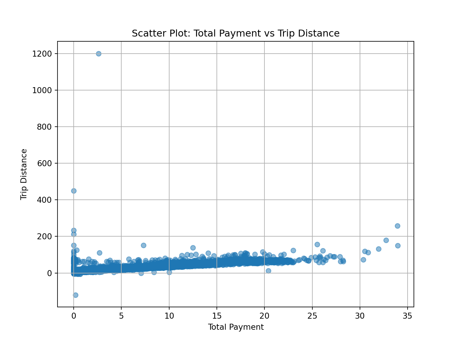
rm_outliers = df[(df['total_amount'] <= 200) & (df['total_amount'] > 0)]

plt.figure(figsize=(8, 6))
plt.scatter(rm_outliers['trip_distance'], rm_outliers['total_amount'], alpha=0.5)
plt.title('Scatter Plot: Total Payment vs Trip Distance')
plt.xlabel('Total Payment')
plt.ylabel('Trip Distance')
plt.grid(True)
plt.show()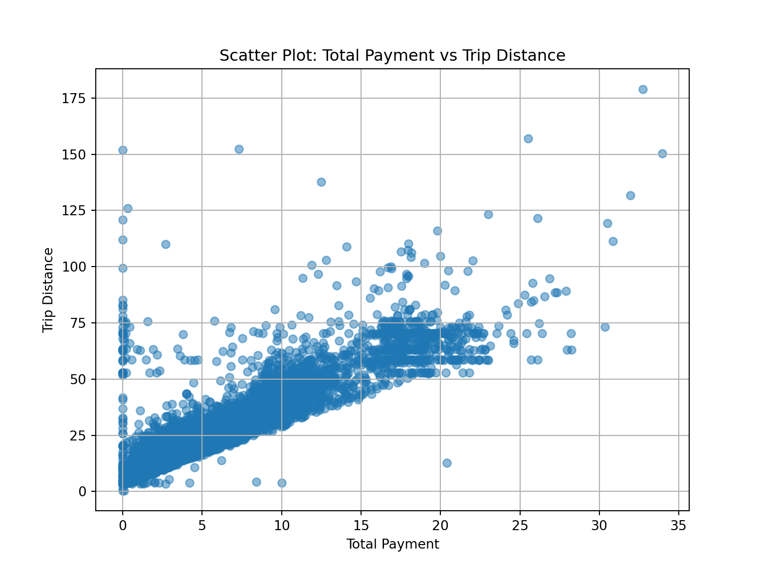
This concludes the Course 2 final assignment